The Cognavitron — hover for details · click to navigate · double-click for full size
Neural Network Movement Models
movement
neural-networks
statistical-modeling
computational-ecology
behavioral-states
hmm
PhD dissertation work: agent-based movement models powered by neural networks, with FMM and HMM behavioral state selection. Von Mises and gamma distributions for turning angle and step length; GA optimization. Applied to puma movement in southern California.
This work dates to my PhD dissertation at Colorado State University, completed in 2006. I mention that not as a historical footnote but because it matters: I have been thinking about neural networks, animal behavior, and landscape ecology for twenty years. The tools have changed beyond recognition — from hand-coded networks fit on desktop workstations to transformer architectures trained on GPU clusters — but the questions I was asking then are the same questions driving my current work. Connectivity. Movement. How animals respond to the landscape they live in. How we build models that are honest about that complexity.
I came to deep learning not through a crash course but through a long arc that started here. That context shapes how I build models, what I think they can and can’t do, and what questions I think are worth asking.
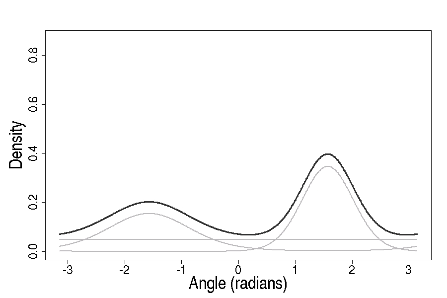
The core idea: use a neural network to model how an animal’s next movement step depends on the surrounding landscape. Step length and turning angle are modeled jointly — step length with a gamma distribution, turning angle with a von Mises distribution. When multiple landscape features compete for influence, the network assigns a mixing weight to each, letting the model capture multi-modal movement decisions. And when behavior itself is a hidden variable — the animal is in one of several unobserved states, each with its own movement dynamics — the model can represent that too, using either a finite mixture or a hidden Markov structure for behavioral state selection.
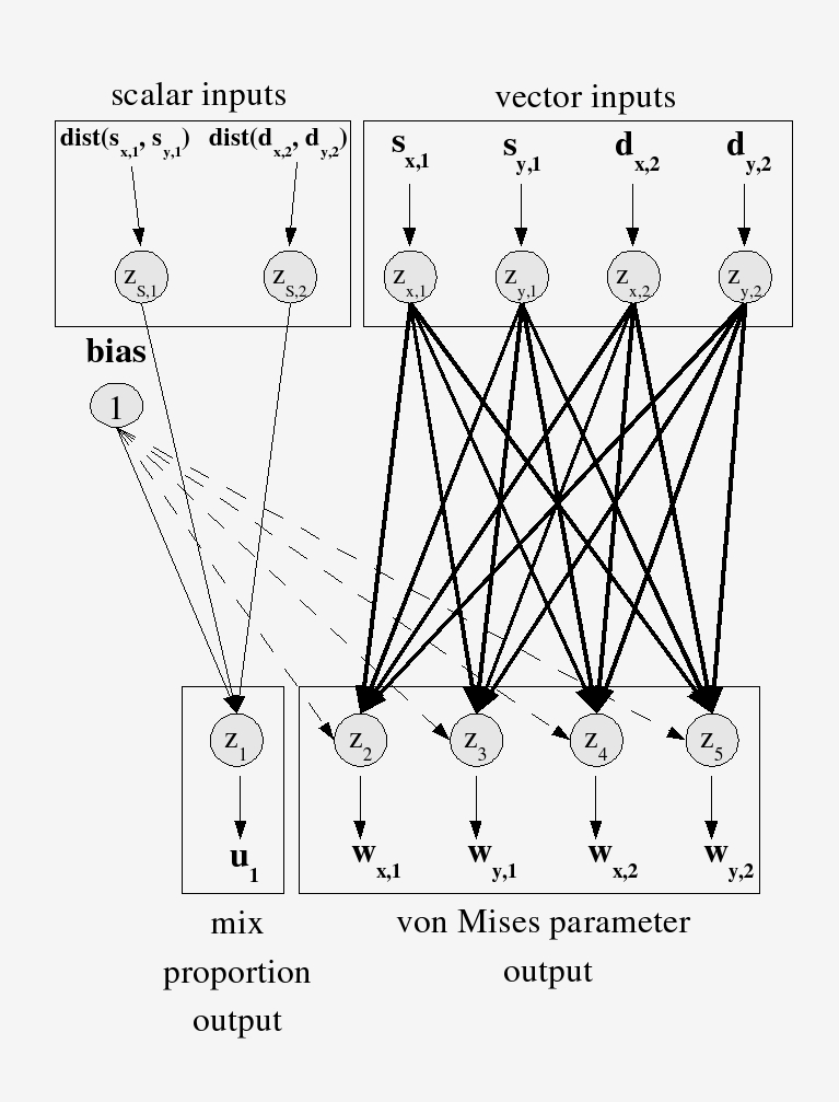
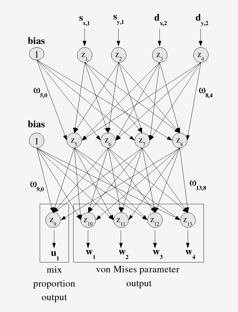
Network Architecture
The network takes landscape inputs and outputs the parameters of probability distributions for turning angle and step length. Turning angle is modeled with a von Mises distribution — the circular analogue of the Gaussian, appropriate for angles. When an animal responds to multiple landscape features, a finite mixture assigns a weight to each component, capturing the multi-modal structure of real movement decisions.
Behavioral State Selection: FMM and HMM
The network architecture solves one problem: how to map landscape inputs to movement distribution parameters. But it leaves a second problem open — what behavioral state is the animal in right now?
A foraging animal and a commuting animal have different movement dynamics even if they’re standing in the same place facing the same landscape. Step lengths differ. Turning angle distributions differ. Any honest movement model has to account for this, and the state itself is never directly observed — only the movement outcomes are. The behavioral state is hidden.
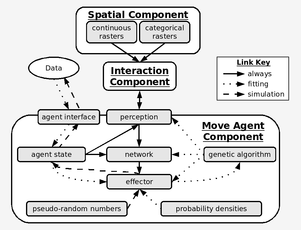
I implemented two alternative model structures for state selection in the move effector:
Finite Mixture Model (FMM). State selection at each step is independent of the previous state — the probability of being in any given behavioral state depends only on the current inputs, not on what the animal was doing a moment ago. This is the simpler, more parsimonious model. It captures the multi-modal structure of movement (multiple possible behaviors at any location) without modeling the transitions between them.
Hidden Markov Model (HMM). State selection is governed by a transition matrix whose entries give the probability of moving from state i to state j at each step. Behavioral persistence is captured explicitly: an animal in a foraging state tends to stay foraging; an animal in a fast-transit state tends to keep moving. The forward algorithm updates state probabilities as the path unfolds.
In both cases, the neural network outputs the parameters of the active state model — including, in the HMM formulation, the elements of the transition matrix itself. The GA then optimizes all of these jointly.
The choice between FMM and HMM is a model selection question, answerable by likelihood-based methods. Running both and comparing was part of the point — the framework was designed to support it.
It is worth noting that the HMM approach I was developing in 2004–2006 is now the dominant paradigm in movement ecology, implemented in widely-used packages such as moveHMM and momentuHMM. The underlying structure — hidden behavioral states, observation-driven emission distributions, Markov transition dynamics — is the same. The implementation pathway here (neural network parameterization, genetic algorithm fitting, agent-based simulation framework) was unconventional then and remains distinctive now.
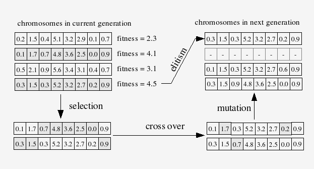
Training with a Genetic Algorithm
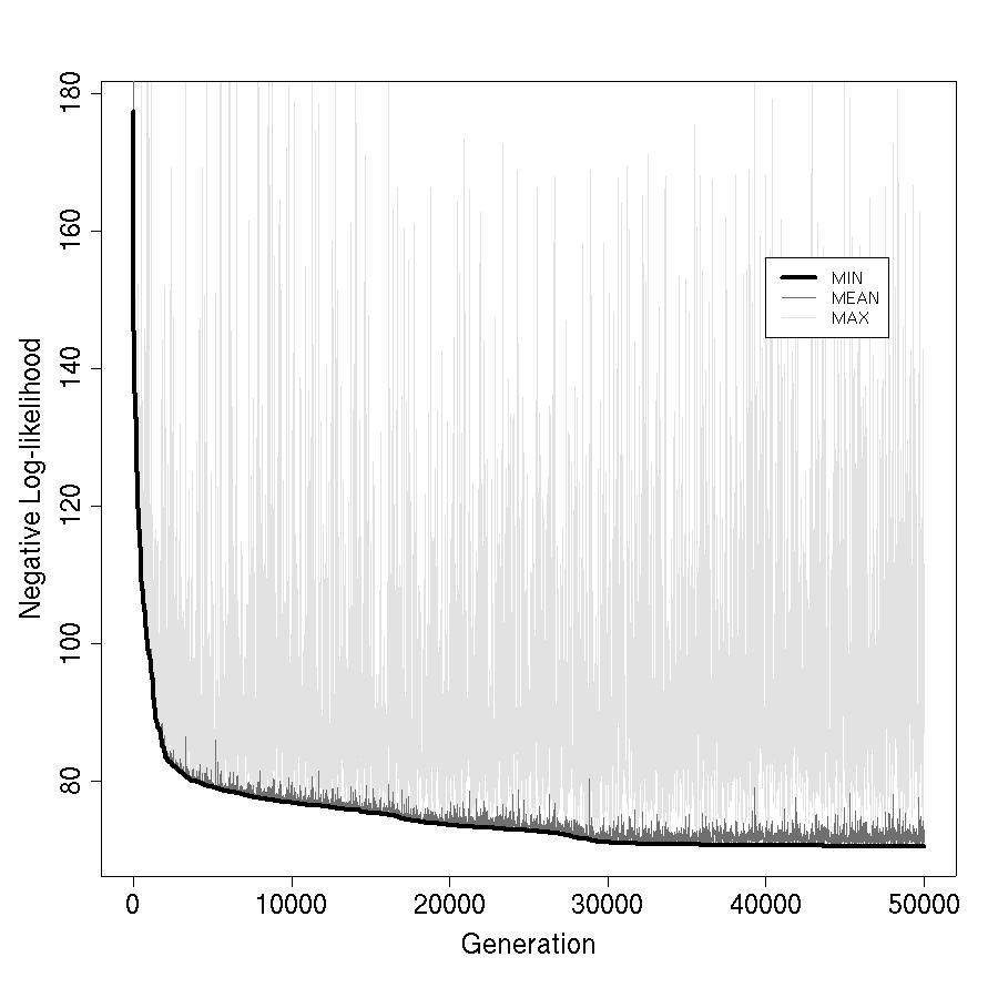
By 2004–2006, gradient-based optimization of neural networks was well-known but practically difficult — vanishing gradients, sensitivity to initialization, and local minima were real problems, especially with small ecological datasets and non-standard output distributions. I trained the networks using a genetic algorithm (GA): a population of candidate weight vectors evolves over generations through selection, crossover, and mutation, with fitness measured by negative log-likelihood on the training data.
Agent-Based Simulation Framework
The fitted network was embedded in an agent-based model (ABM) to simulate animal movement through heterogeneous landscapes. The GA is not just a training tool — it is part of the model architecture, iterating within the ABM to fit parameters to observed movement data for each individual animal.
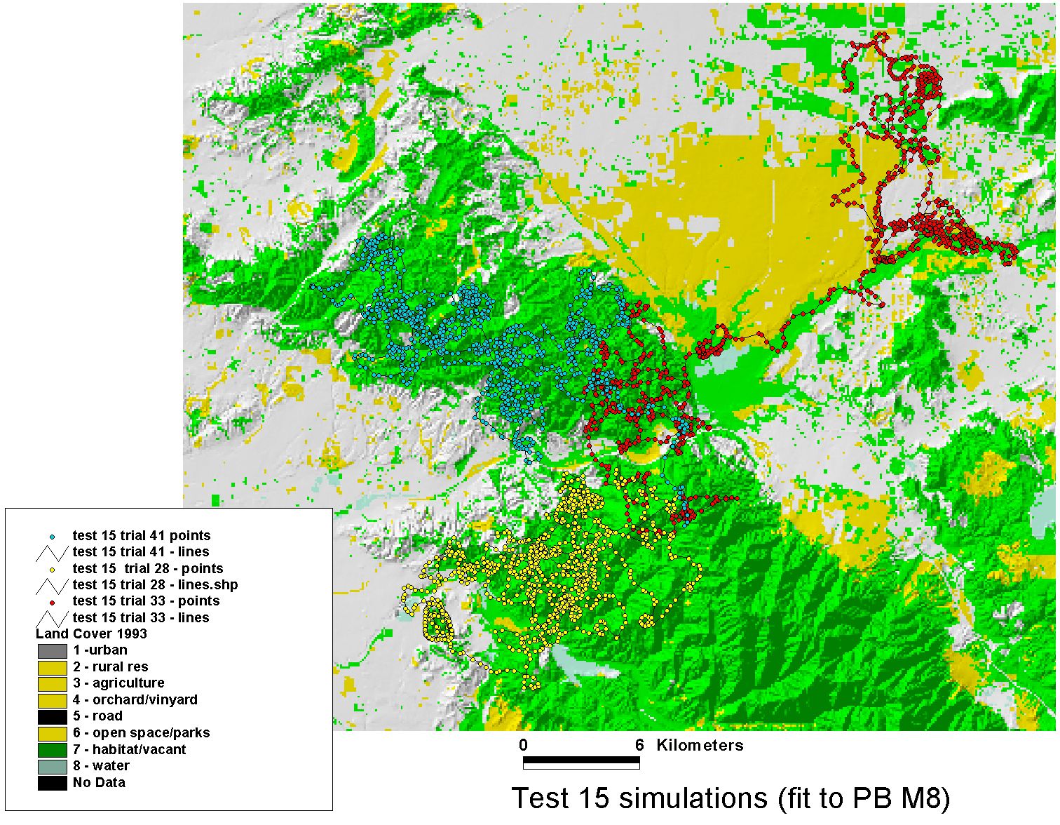
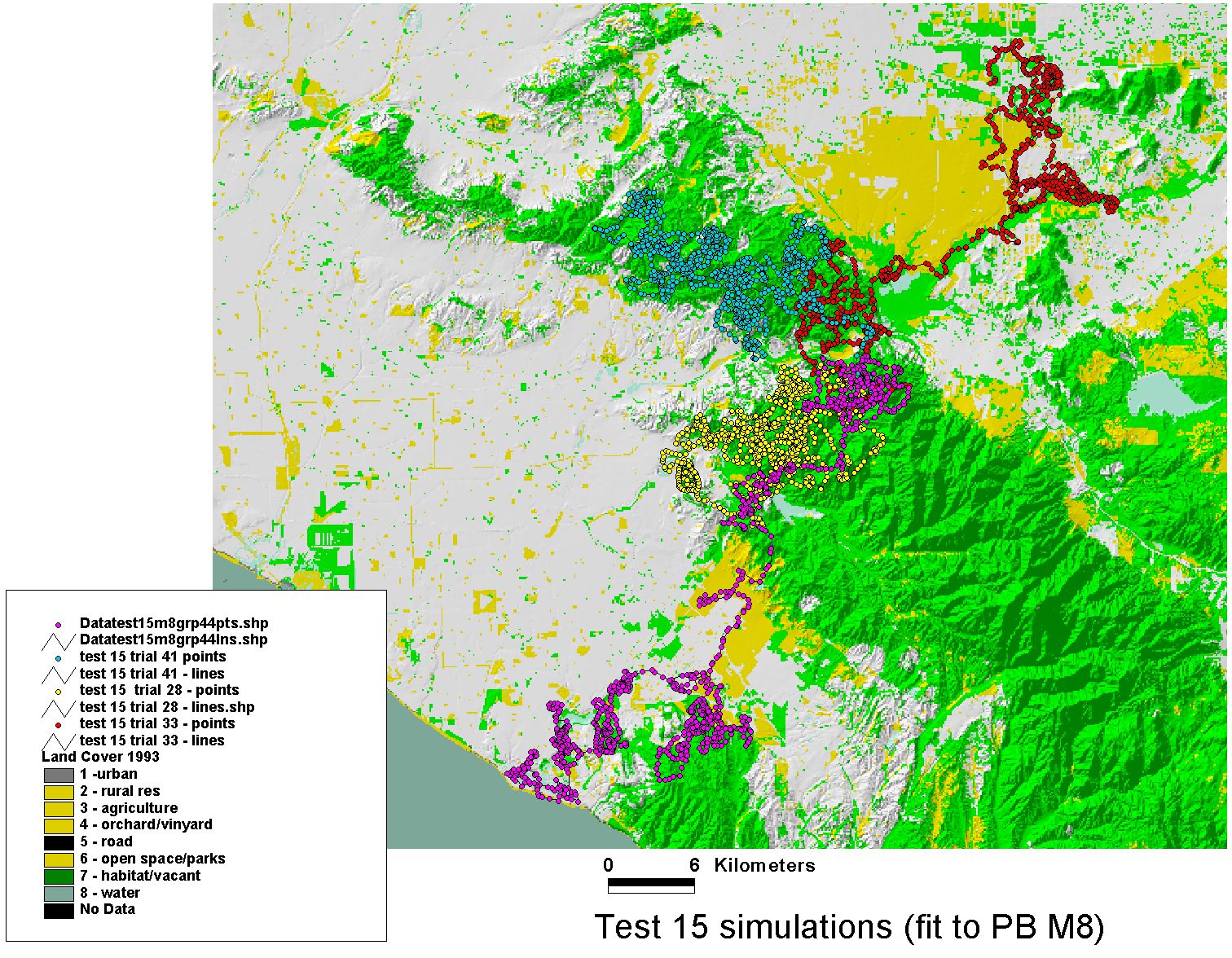
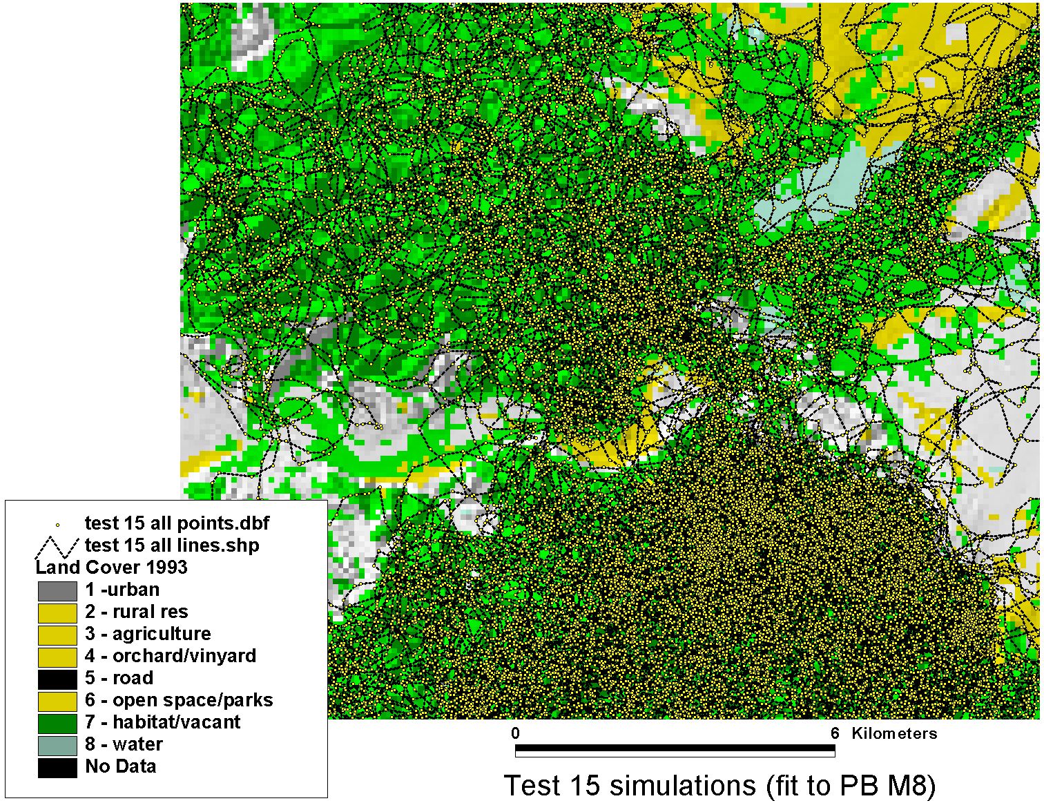
Simulations — Puma Movement in Southern California
The fitted model was validated by simulation: run the trained agent forward through the landscape and compare the simulated paths to observed movement data. The puma data used here were generously shared by Paul Beier (Northern Arizona University), whose long-term field work on mountain lion (Puma concolor) movement and landscape connectivity in southern California provided an ideal test case — a large-bodied carnivore navigating a highly fragmented urban-wildland matrix.
Papers
Tracey JA, Zhu J, Boydston E, Lyren L, Fisher RN, Crooks KR (2013). Mapping behavioral landscapes: a finite mixture modeling approach. Ecological Applications 23(3): 654–669. (Cover article) https://doi.org/10.1890/12-0687.1
Tracey JA, Zhu J, Crooks KR (2011). Modeling and inference of animal movement using artificial neural networks. Environmental and Ecological Statistics 18(3): 393–410. https://doi.org/10.1007/s10651-010-0138-8
Tracey JA, Zhu J, Crooks KR (2005). A set of nonlinear regression models for animal movement in response to a single landscape feature. Journal of Agricultural, Biological, and Environmental Statistics 10(1): 1–18. https://doi.org/10.1198/108571105X29056
Tracey JA (2006). Agent-based movement models and landscape connectivity. Ph.D. Dissertation, Colorado State University.
Tracey JA (2004). Models for Animal Movement in Response to Landscape Features. M.S. Thesis in Biometry, University of Wisconsin – Madison.