The Cognavitron — hover for details · click to navigate · double-click for full size
Ivory-billed Woodpecker Habitat Network Modeling
2026-06-17
The ivory-billed woodpecker (Campephilus principalis) was presumed extinct after 1944. Then, in 2004, video footage from the Big Woods of Arkansas suggested it might not be. That possibility triggered a serious search effort under the Federal Endangered Species Act.
If you are going to search for a bird that may or may not still exist, you need to know where to look. And if there are remnant individuals, you need to understand whether the landscape can actually support a viable population — whether the patches of suitable habitat are connected enough to matter.
This project addressed both questions using a habitat filter model and graph-theoretic approach to habitat network modeling. I did this work in collaboration with Barry Noon (Colorado State University) and Curt Flather (US Forest Service). THe network analysis was funded by the US Fish and Wildlife Service Lower Mississippi Valley Joint Venture Office.
Habitat Filter Model
What makes a patch of forest usable as ivory-billed woodpecker habitat? The answer had to be reconstructed from history. James Tanner’s monograph — based on meticulous field observations of the Singer Tract population in Louisiana in the 1930s — remains the primary ecological reference for the species. Tanner documented the food base (large beetle larvae in recently dead hardwood timber), the necessary forest structure (large trees, high basal area), and the disturbance regime (low-level, gap-producing disturbance maintaining a continuous supply of recently dead wood) that sustained the last known breeding population.
The filter model — developed with Curt Flather (USFS Rocky Mountain Research Station), Barry Noon (Colorado State University), Robert Sheffield, and Scott Knowles — is a multi-node decision tree applied to US Forest Service Forest Inventory and Analysis (FIA) plot data. FIA plots sample forest condition at tens of thousands of locations across the US landscape, distributed in a systematic hexagonal grid. Each node in the decision tree tests a measurable stand attribute: plot status, land cover class, forest type, physiographic class, stem densities across size classes, standing dead wood volume, years since last disturbance, forest patch size, and habitat amount within the surrounding neighborhood. The filter has two sub-models: a habitat filter that screens for basic stand structure, and a landscape context sub-model that evaluates patch size and habitat continuity for plots that pass the structural screen.
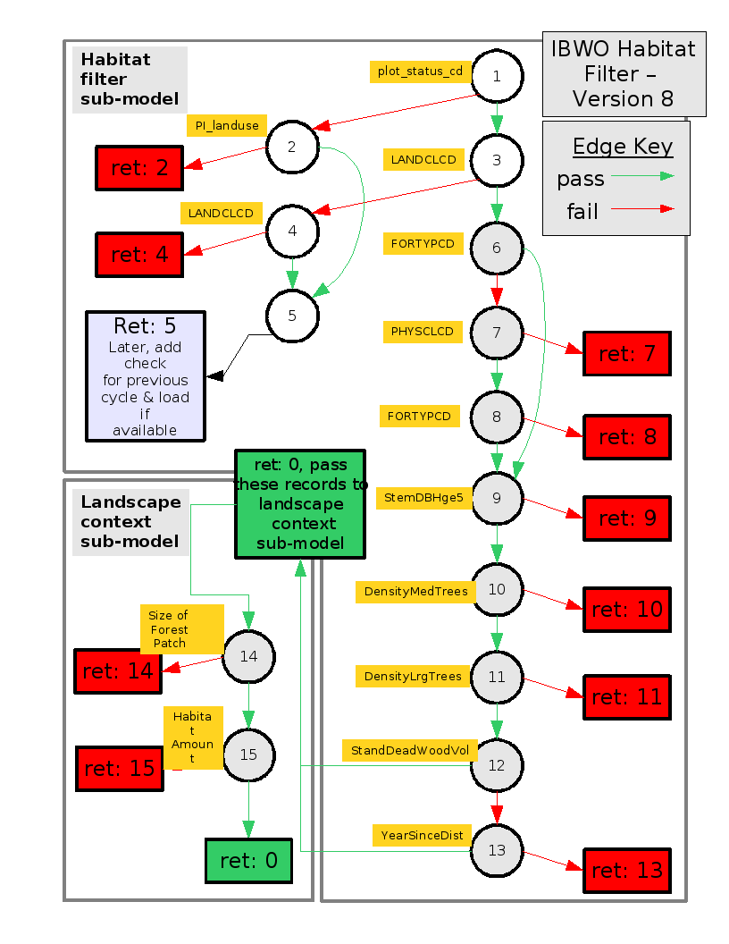
Two versions of the filter were implemented. The deterministic version used fixed threshold values at each node — a plot either passed or failed. The stochastic version drew filter values from probability distributions estimated from Tanner’s Singer Tract data, producing a habitat probability at each FIA plot rather than a binary classification. Multiple stochastic runs generated an ensemble of habitat maps, capturing uncertainty in how Tanner’s historical observations translate to present-day range-wide conditions.
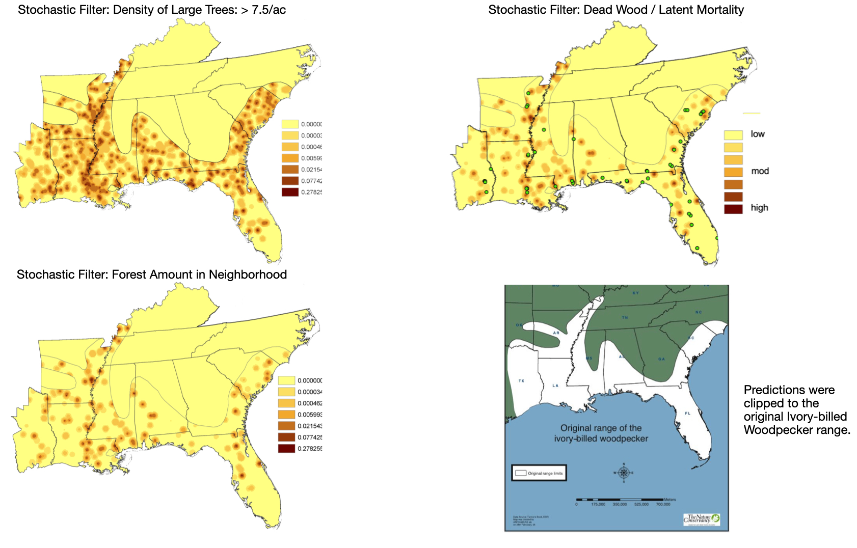
The model was validated against two independent sources: the Big Woods of Arkansas search area (site of the 2004 video footage) and the set of post-1944 sighting reports compiled from the ornithological literature. FIA plots near documented sightings scored higher on average than random locations across the range — a meaningful signal given the coarse resolution of FIA data and the age of the ecological baseline.
Plots with a greater-than-zero probability of being habitat became nodes in the connectivity network. The search originated the title of the IALE 2009 presentation this work was published in: Searching for Where to Search: Sifting Forest Inventories for Potential Ivory-billed Woodpecker Habitat.
Network Construction
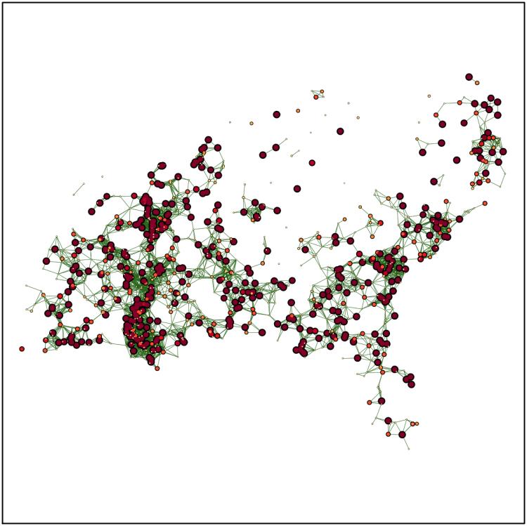
In the graph-theoretic approach, habitat patches are nodes and potential movement corridors between them are edges. Two nodes were connected by an edge if they fell within a maximum distance threshold. We analyzed three thresholds — 30 km, 60 km, and 100 km — bracketing estimates of maximum dispersal distance derived from allometric relationships for large-bodied woodpeckers.
Each edge was assigned a weight representing the cost of movement between nodes, as a function of distance. The standard “classical” formulation for edge weights is one-dimensional — it treats dispersal as a process along a line. We proposed an alternative 2-dimensional formulation that treats dispersal as a process across an area, which is geometrically more appropriate for a landscape. The two formulations lead to meaningfully different results: the 2D model favors many short moves over one long move, while the 1D model is more permissive of long-distance jumps. We argued the 2D formulation is more biologically realistic, and present results primarily from that model.
We also incorporated a gravity model formulation to estimate potential flux of individuals between nodes — weighting movement by both distance and habitat quality at the source and destination. The network was implemented in Python using the NetworkX library.
What the Network Revealed
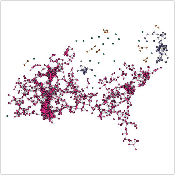
Component Structure
At the 30 km threshold, the network fragments into many disconnected components — patches of habitat too far apart to be reached in a single dispersal event. As the threshold increases to 60 and 100 km, components merge and the network becomes increasingly connected. At 60 km, two large clusters dominate: one along the lower Mississippi River and one along the Atlantic coastal plain. These correspond to the areas most frequently identified in post-1944 sighting reports.
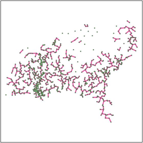
Network Backbone
The minimum spanning tree identifies the set of edges that connect all nodes at minimum total cost — the skeletal backbone of the network. For conservation planning, this highlights which movement corridors are load-bearing: lose them, and the network falls apart.
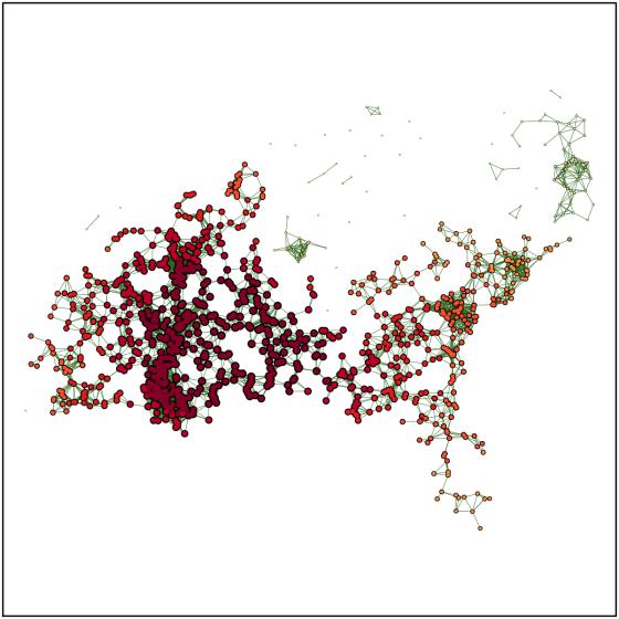
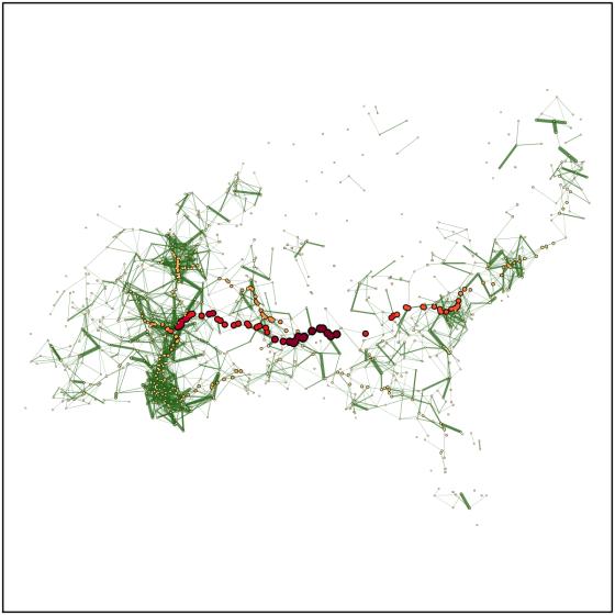
Centrality and Connectivity
We computed multiple centrality metrics for each node: degree (number of connections), closeness (how quickly a node can reach all others), and betweenness (how often a node lies on shortest paths between other nodes). Betweenness centrality is particularly relevant for conservation — high-betweenness nodes are structural bridges, and their loss disproportionately fragments the network.
Contributions
Beyond the ivory-billed woodpecker application, we made three methodological contributions to graph-theoretic landscape analysis:
- A 2D formulation of edge weights — more geometrically appropriate for spatial dispersal across a landscape than the standard 1D exponential model.
- Gravity model flux — incorporating habitat quality at both source and destination nodes to estimate potential movement between patches.
- Systematic comparison of network algorithms — degree, closeness, betweenness, k-cores, minimum spanning trees, and flux metrics evaluated together, providing a template for multi-metric landscape network analysis.
The approach is general and was designed to be applicable to other species with broad geographic ranges — particularly useful for forecasting how habitat loss and climate-driven range shifts will alter landscape connectivity.
Report
Tracey JA, Flather CH, Noon BR (2010). Network Analysis of Potential Ivory-billed Woodpecker Habitat. Prepared for the US Fish and Wildlife Service, Lower Mississippi Valley Joint Venture Office. 30 December 2010.