The Cognavitron — hover for details · click to navigate · double-click for full size
Bobcat Movement — Finite Mixture Models
2026-06-17
Where an animal goes tells you part of the story. How it moves through different parts of the landscape tells you something deeper — what it is responding to, what it is avoiding, what it is ignoring. A bobcat crossing a road at speed is doing something different than a bobcat hunting the edge of a chaparral patch, even if both movements appear as points on a GPS track.
This project developed a method for extracting those behavioral distinctions from GPS movement data and mapping them across the landscape — producing what we called a behavioral landscape: a map not of where the animal went, but of how the landscape shaped its behavior at every location.
The work was a collaboration with Jun Zhu (University of Wisconsin–Madison), Erin Boydston, Lisa Lyren, and Robert Fisher (USGS Western Ecological Research Center), and Kevin R. Crooks (Colorado State University). The study system was GPS-tracked bobcats (Lynx rufus) in coastal southern California — a heavily urbanized, fragmented landscape where animals must navigate a matrix of natural habitat, roads, and development. The paper was selected for the cover of Ecological Applications 23(3), 2013.
The Behavioral Landscape Concept
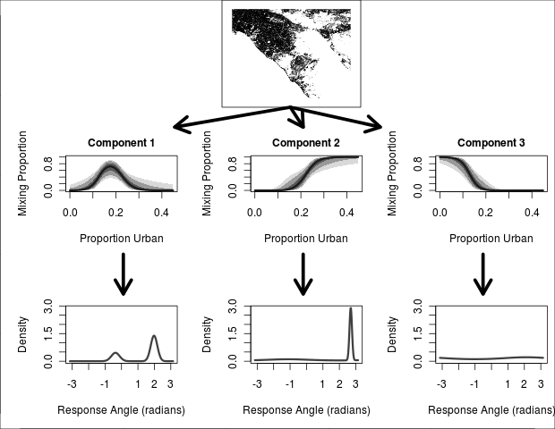
The core idea is that an animal’s movement at any location is a behavioral response to the landscape features around it. Those responses fall into a small number of qualitatively distinct modes — foraging, resting, commuting, avoiding — each with a characteristic statistical signature in the step length and turning angle distributions of the GPS track.
A finite mixture model (FMM) decomposes the movement data into these latent behavioral components without requiring the analyst to specify them in advance. Each GPS step is assigned a probability of belonging to each component, and the landscape covariates associated with each component reveal what the animal is responding to.
The result is a map: for every point in the landscape, what behavioral mode does this location tend to elicit? That is the behavioral landscape.
Study System
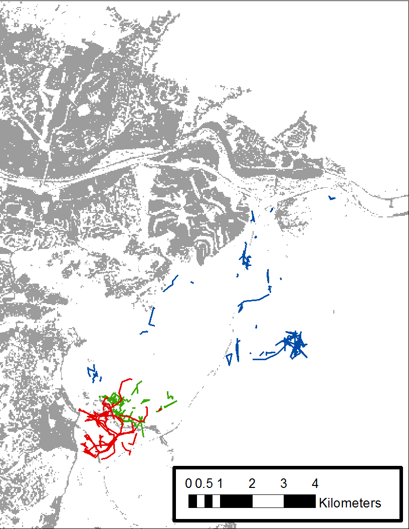
Three GPS-tracked bobcats in coastal southern California provided the movement data. The landscape is a mosaic of natural chaparral and coastal scrub, fragmenting urban development, highways, and open space preserves — a challenging environment for a medium-sized predator with a large home range.
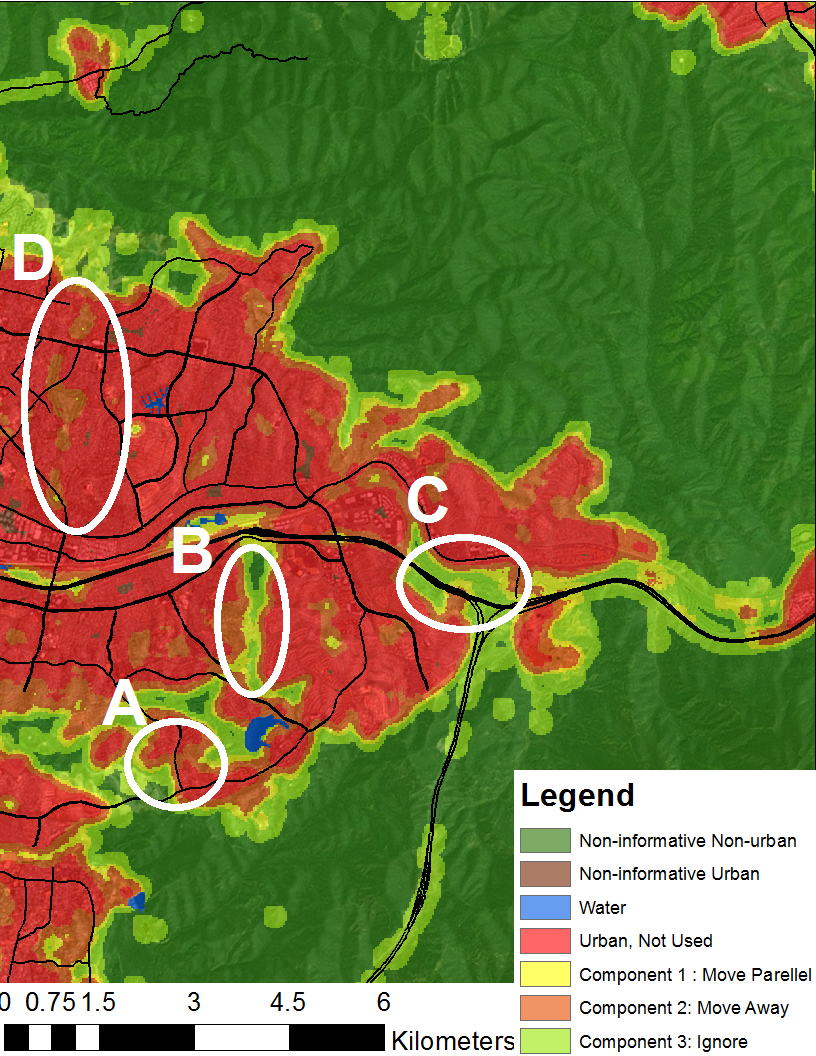
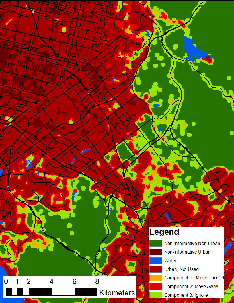
Behavioral Landscape Maps
Fitting the finite mixture model to each individual’s GPS data and associating the behavioral components with landscape covariates produced a continuous map of behavioral response across the landscape. Each location on the map is assigned the behavioral mode most likely to be elicited there — based on what the animal actually did when it was in places with similar landscape characteristics.
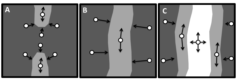
Three behavioral components emerged consistently: movement parallel to landscape features (corridor-following), movement away from features (avoidance), and non-informative movement (the animal ignoring the feature). Roads, habitat edges, and urban development each produced distinct patterns of behavioral response.
Papers
Tracey JA, Zhu J, Boydston E, Lyren L, Fisher RN, Crooks KR (2013). Mapping behavioral landscapes: a finite mixture modeling approach. Ecological Applications 23(3): 654–669. https://doi.org/10.1890/12-0687.1
Ruell EW, Riley SPD, Douglas MR, Antolin MF, Pollinger JR, Tracey JA, Lyren LM, Boydston EE, Fisher RN, Crooks KR (2012). Urban habitat fragmentation and genetic population structure of bobcats in coastal southern California. The American Midland Naturalist 168(2): 265–280. https://doi.org/10.1674/0003-0031-168.2.265
Boydston EE, Tracey JA, Preston KL, Rochester CJ, Fisher RN (2018). Modeling resource selection of bobcats (Lynx rufus) and vertebrate species distributions in Orange County, southern California. USGS Open-File Report 2018-1095. https://doi.org/10.3133/ofr20181095